Linux PRNG Internals
An article on Linux Pseudo-Random Number Generator Internals
Linux Pseudo-Random Number Generator (PRNG) Internals
Introduction
I came across the slides of a presentation by J. Donenfeld on Linux/OpenBSD Kernel Random Number Generators (RNG). In one of the slides, a weakness in the generator has been mentioned. The original design is based on the paper “Twisted GFSR Generators” by Matsumoto and Kurita. 92' paper describes an elegant way to make use of a generalized feedback shift register to generate a key stream. However, the implementation did not follow the paper’s assumptions that makes the generator vulnerable. Here is a brief study of the PRNG included in the Linux Kernel for the curious.
Fundamentals of LFSR Sequences
Linear Feedback Shift Registers are common building blocks of stream ciphers and PRNG’s. They have been studied extensively for instance in Shift Register Sequences, Golomb (RIP). I must admit, Golomb’s algorithm for generating DeBruijn sequences is far more interesting than LFSR’s. In Algebraic Shift Register Sequences, Goresky, one may find the study not only sequences over finite fields but also p-adic sequences over integers.
An LFSR example from Wikipedia is the following.

At each clock, the feedback is calculated by XOR’ing the values from cells 11, 13, 14 and 16 and the result is placed in cell 1. First equation that defines the register is the difference equation or linear recurrence relation.
\[ s_{n} = s_{n-11} + s_{n-13} + s_{n-14} + s_{n-16}, \quad \forall n \in \mathbb{Z}, n \geq 16 \]In the polynmoial ring \( \mathbb{F}_2[x] \), the connection polynomial is the following:
\[ f(x) = \sum_{i=0}^{n} a_i x^i \quad where\quad a_i \in \mathbb{F}_2 \]\(n\) is called the degree of \( f(x) \) and it is the number of cells. The polynomial \(f(x)\) is called irreducible if \( f(x) = g(x)h(x) \) then either \(g(x)\) or \(h(x)\) is a unit in our case. Therefore, we can assume \( f(x) \) is monic that is \( a_n = 1 \). Let \( \alpha \in \overline {\mathbb{F}_2} \) be a root of \(f(x)\) s.t. \(f(\alpha) = 0 \). Then the period of the sequence is equal to the order of \(\alpha\) s.t. \( \alpha^{ord(\alpha)} = 1 \) holds. Note that \( \alpha \neq 0 \) since \( f(x)\) is not divisible by \( x \) (ie. \( a_0 \neq 0 \)) where in the that case \( f(x) \) is reducible. Moreover, if the initial values in the cells are adjusted appropriately, the i'th element of the sequence can be calculated by the following:
\[ Tr_1^n(\theta \alpha^{-i}) = \sum_n \sigma_n(\theta \alpha^{-i}), \theta \in \overline{\mathbb{F}_2} \]
where \(Tr_1^n(x)\) is the trace of \(x\) and \( \sigma_n \) is the Frobenius Automorphism of the Finite Field Extension of degree \(n\) with \( \sigma_n(x) = x^{p^n} \). Let’s verify this claim.
\[ s_{n} = s_{n-11} + s_{n-13} + s_{n-14} + s_{n-16} \]\[ Tr(\theta\alpha^{-n}) = Tr(\theta\alpha^{-n+11}) + Tr(\theta\alpha^{-n+13}) + Tr(\theta\alpha^{-n+14}) + Tr(\theta\alpha^{-n+16}) \]\[ 0 = Tr(\theta\alpha^{-n} + \theta\alpha^{-n+11} + \theta\alpha^{-n+13} + \theta\alpha^{-n+14} + \theta\alpha^{-n+16}) \]\[ 0 = Tr( (\theta\alpha^{-n}) (1 + \alpha^{11} + \alpha^{13} + \alpha^{14} + \alpha^{16})) \]\[ 0 = Tr( (\theta\alpha^{-n}) f(\alpha)) \]\[ 0 = Tr(0) \]This explains the why the period of the sequence is related to the order of the root of \( f(x) \). Finally, if \( \alpha \) is primitive, then the period is \( 2^n -1 \) which is one less than the period of DeBruijn sequences. The missing value is all zeros and an LFSR outputs all zeros if the initial value in the cells are all zeroes, then the period becomes 1.
Generalized Feedback Shift Registers [LP73]
Information on GFSR's can be found in the paper by Lewis and Payne. There are two important characteristics that define GFSR's:
- Base field is extented to arbitrary word size,
- Connection polynomial is a trinomial.
So the first one is basically making each cell match the wordsize of the machine that we are working on. This makes XOR operations easy to implement in high-level languages, also improves caching.
A trinomial is a polynomial in the form of \( f(t) = t^n + t^m + 1, n,m \in \mathbb{Z}^+, n \gt m \gt 0 \). Coefficient of the middle term might be non-one in other definitions but we are going with all 1's here. The second characteristic therefore simplifies the algorithm pretty much. For instance, in the paper by Matsumoto and Kurita, the following algorithm is defined:
- \( l \leftarrow 0 \)
- Set \( x[0], x[1], \ldots, x[n-1] \) to some suitable initial values,
- Output \( x[l] \),
- \( x[l] \leftarrow x[(l+m)\ mod\ n] \oplus x[l] \)
- \( l \leftarrow (l+1)\ mod\ n \)
- Goto Step 3.
In the case \(f(t)\) is primitive, the period of the sequence is \(2^n-1\). It is an interesting problem to find such primitive polynomials given \(n,m\) and it is studied extensively.
Twisted GFSR [MK92]
In the 1992 paper by Matsumoto and Kurita, a twisted version of the GFSR is defined to increase the period of the sequence.
In the above algorithm, Step 4 is replaced by the following:
\[ x[l] \leftarrow x[(l+m)\ mod\ n] \oplus (x[l] \gg 1) \oplus a' \]where \( a' \) is zero if LSB of x[l] is zero, and it is the constant \(a \in \mathbb{F}_{2^w}\) otherwise. \( w \) is defined to be the degree of the extension of the base field, usually one of 16, 32 or 64.
The modification can be seen as in the following connection polynomial.
\[ x_{l+n} : = x_{l+m} \oplus x_l A, \quad l=0,1,\ldots \]where \(A\in GL(w, \mathbb{F}_2) \), a non-singlar matrix with elements from the base field and \(x[l]\) is a row vector. It is chosen to be in the following form for wordsize 8:
\[ A = \left( \begin{matrix} a_7 & 1 & 0 & 0 & 0 & 0 & 0 & 0 \\ a_6 & 0 & 1 & 0 & 0 & 0 & 0 & 0 \\ a_5 & 0 & 0 & 1 & 0 & 0 & 0 & 0 \\ a_4 & 0 & 0 & 0 & 1 & 0 & 0 & 0 \\ a_3 & 0 & 0 & 0 & 0 & 1 & 0 & 0 \\ a_2 & 0 & 0 & 0 & 0 & 0 & 1 & 0 \\ a_1 & 0 & 0 & 0 & 0 & 0 & 0 & 1 \\ a_0 & 0 & 0 & 0 & 0 & 0 & 0 & 0 \\ \end{matrix} \right) \]This explains the significance of the least significant bit of \( x[l] \). If the LSB is on, then the last row of \(A\) is added.
\[ a = \sum_{i=0}^{w-1} a_n x^i \]Let \( \varphi_A(t) \) be the characteristic polynomial of \(A\).
\[ \varphi_A(t) = det(tI_w - A) \]where \(I_w\) is the \(w \times w\) identity matrix. Then, Theorem 1 in the paper proves the following:
\( \varphi_A(t^n+t^m)\) is a primitive polynomial if and only if the period of the sequence is \(2^{nw} -1 \)
In this case, the sequence is called m-TGFSR sequence of maximal length. We are left with finding such parameters \(n,m\) where the connection polynomial stays irreducible with a primitive root. Theorem 2 provides the conditions exactly for this to hold.
- The polynomial \(\varphi_A(t)\) is irreducible,
- The polynomial \( t^n + t^m + \eta \) is primitive over \( \mathbb{F}_{2^w} \)
where \( \eta \) is a root of \( \varphi_A(t) \) s.t. \(\varphi_A(\eta) = 0 \) holds. Now the problem boils down to finding a degree \(n\) extension of \( \mathbb{F}_{2^w} \). Fortunately, Proposition 1 guides us through that maze.
Let \( \eta \) be an element of \(\mathbb{F}_{2^w}\). The polynomial \(f(t) = t^n+t^m+\eta\) has an even number of irreducible factors hence is not irreducible if one of the followings hold.
- \( n \equiv \pm 3\ mod\ 8, w:odd, m:even, m \nmid 2n \),
- \( n \equiv \pm 3\ mod\ 8, w:odd, m:odd,\ n-m \nmid 2n \),
- \( n:even, m:even\),
- \( n:even, n\neq 2m,\ and\ nm \equiv 0,2\ mod\ 8 \),
- \( n:even, n\neq 2m, nm \equiv 4,6\ mod\ 8, w:even \)
The Linux PRNG - Theory of Operation [GPR06], [LRSV12]
In this section, I'll follow the 2012' paper The Linux Pseudorandom Number Generator Revisited by Lacharme, Rock, Strubel and Videau.
The Linux PRNG is comprised of several components. First component is the entropy collection. Various entropy sources provide entropy and estimations regarding to these sources are as follows:
The frequency of the timer interrupt is defined at build time by the HZ parameter in the kernel source, and generally ranges between 100 to 1000 ticks per second [CRKH05, Ch. 7]. These values provide much less than 32 bits of entropy each. As shown in [GPR06, Table 1], the maximal entropy of the 32-bit num value is 8 bits for keyboard events, 12 bits for mouse events, 3 bits for hard drive events, and 4 bits for interrupts.
I've borrowed the following diagram to explain the PRNG better. The entropy collected is fed into an input pool which is the next component in the production line. To avoid directly using the collected data, a mixing function is employed to prevent correlation attacks feasible. The input pool is defined to be 128 32-bit words (4k bits) in the current implementation but it was smaller before so don't get confused if you see smaller pools in the diagrams.

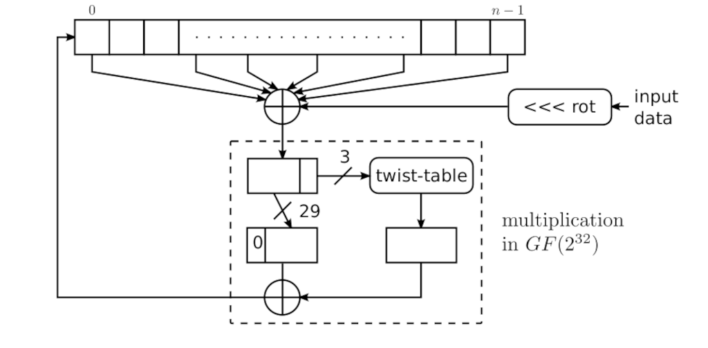
In the paper, the mixing function is depicted as in the following diagram. The input is on the right that is 32bits wide. The Twisted GFSR is shown at the top with 32bits wide cells. The values of the cells of the taps of the twisted GFSR are XOR'd with the rotated input data. Then, the result is multiplied by the last coefficient which is \( \in \mathbb{F}_{2^{32}} \). Final result is fed into the zero'th cell, shifting the GFSR to the right.
The problem we are left with is the entropy transfer to the output pool and the output itself. The following figure in [GPR06] depicts the transfer operation. There are two stages in this operation. First, the feedback then the extraction. The topmost row is the input pool. The input pool is hash'd with SHA1. The result is 5*32bits or 20 bytes and it is mixed back into the input pool.

To understand this operation, we need to refer to the 2006 paper by Gutterman, Pinkas and Reinman. Authors of the paper reverse engineered the theory of operation and presented it in the following diagram.

The operation starts with hash of the LSB 16 dwords. LSB byte of the output added to i'th cell. Next, the MSB 16 dwords are hash'd and 3rd and 5th bytes of the hash are added to i-2'th and i-1'th cells. The operation continues in this fashion. The details are in the folowing pseudo-algorithm however i is now j.
extract(pool, nbytes, j)
 while nbytes > 0
       tmp := SHA1(pool[0..15])
       add(pool, j, tmp[0])
       tmp := SHA1(pool[16..31])
       add(pool, (j-1 mod 32), tmp[2])
       add(pool, (j-2 mod 32), tmp[4])
       tmp := SHA1(pool[((j-2-15) mod 32) .. ((j-2) mod 32)])
       tmp := folding(tmp[0..4])
       output(tmp, min(nbytes, 10))
       nbytes -= min(nbytes,10)
       j -= 3 mod 32
 end while
What we have learned from the algorithm is the minimum number of output bytes is 10. The folding operation is a little different from what you might assume. It is not symmetric.
\[ folding : \mathbb{F}_2^{32} \times \mathbb{F}_2^{32} \times \mathbb{F}_2^{32} \times \mathbb{F}_2^{32} \times \mathbb{F}_2^{32} \rightarrow \mathbb{F}_2^{32} \times \mathbb{F}_2^{32} \times \mathbb{F}_2^{16} \]\[ (x_0,x_1,x_2,x_3,x_4) \rightarrow (x_0 \oplus x_3, x_1 \oplus x_4, x_2[0..15] \oplus x_2[16..31]) \]One interesting fact is that while the j-2'th cell effects the current output, j-1 and j'th cells do not. There are questions in my mind like where j starts from or when the cells are rotated since the input to the last SHA1 is not contiguous in memory.
Efficient Implementation of Field Operations
Before looking into the parameter selection, let's have a peek into the implementation of the mixing function. This will help us to understand how certain choices of parameters effect the implementation.
The following is revision 9e95ce279fa611226a1ab0dff1c237c080b51b60 from v2.6.12. This is the earliest I can go these days as git repo doesn't go beyond v2.6.12.
 286 static struct poolinfo {
 287         int poolwords;
 288         int tap1, tap2, tap3, tap4, tap5;
 289 } poolinfo_table[] = {
 290         /* x^128 + x^103 + x^76 + x^51 +x^25 + x + 1 -- 105 */
 291         { 128,  103,    76,     51,     25,     1 },
 292         /* x^32 + x^26 + x^20 + x^14 + x^7 + x + 1 -- 15 */
 293         { 32,   26,     20,     14,     7,      1 },
 ... omitted for brevity ...
 322

... omitted for brevity ...

 451 static void __add_entropy_words(struct entropy_store *r, const __u32 *in,
 452                                 int nwords, __u32 out[16])
 453 {
 454         static __u32 const twist_table[8] = {
 455                 0x00000000, 0x3b6e20c8, 0x76dc4190, 0x4db26158,
 456                 0xedb88320, 0xd6d6a3e8, 0x9b64c2b0, 0xa00ae278 };
 457         unsigned long i, add_ptr, tap1, tap2, tap3, tap4, tap5;
 458         int new_rotate, input_rotate;
 459         int wordmask = r->poolinfo->poolwords - 1;
 460         __u32 w, next_w;
 461         unsigned long flags;
 462
 463         /* Taps are constant, so we can load them without holding r->lock.  */
 464         tap1 = r->poolinfo->tap1;
 465         tap2 = r->poolinfo->tap2;
 466         tap3 = r->poolinfo->tap3;
 467         tap4 = r->poolinfo->tap4;
 468         tap5 = r->poolinfo->tap5;
 469         next_w = *in++;
 470
 471         spin_lock_irqsave(&r->lock, flags);
 472         prefetch_range(r->pool, wordmask);
 473         input_rotate = r->input_rotate;
 474         add_ptr = r->add_ptr;
 475
 476         while (nwords--) {
 477            w = rol32(next_w, input_rotate);
 478            if (nwords > 0)
 479               next_w = *in++;
 480            i = add_ptr = (add_ptr - 1) & wordmask;
 481            /*
 482             * Normally, we add 7 bits of rotation to the pool.
 483             * At the beginning of the pool, add an extra 7 bits
 484             * rotation, so that successive passes spread the
 485             * input bits across the pool evenly.
 486             */
 487            new_rotate = input_rotate + 14;
 488            if (i)
 489              new_rotate = input_rotate + 7;
 490            input_rotate = new_rotate & 31;
 491
 492            /* XOR in the various taps */
 493            w ^= r->pool[(i + tap1) & wordmask];
 494            w ^= r->pool[(i + tap2) & wordmask];
 495            w ^= r->pool[(i + tap3) & wordmask];
 496            w ^= r->pool[(i + tap4) & wordmask];
 497            w ^= r->pool[(i + tap5) & wordmask];
 498            w ^= r->pool[i];
 499            r->pool[i] = (w >> 3) ^ twist_table[w & 7];
 500         }
 501
 502         r->input_rotate = input_rotate;
 503         r->add_ptr = add_ptr;
 504
 505         if (out) {
 506           for (i = 0; i < 16; i++) {
 507              out[i] = r->pool[add_ptr];
 508              add_ptr = (add_ptr - 1) & wordmask;
 509           }
 510         }
 511
 512         spin_unlock_irqrestore(&r->lock, flags);
 513 }
So how does the above function do the algebra over the field? The operation above apart from rotations looks like the following.
\[ s_0 = \eta^{-3}(s_{n+tap1} \oplus s_{n+tap2} \oplus \ldots \oplus s_{n+tapm} \oplus rol32(entropy\_in, j))\]where m is the number of taps, \( \eta \in \mathbb{F}_{2^{32}} \) is a root of a polynomial of degree 32, rol32 is rotate left 32bits, entropy_in is the input entropy and j is the number of rotations to be applied. The elements in the cells are assumed to be written in polynomial basis \( {1, \eta, \eta^2, \ldots, \eta^{31} } \) in order this to work. This implementation aligns with the paper [LP73] and TGFSR modification in [MK92]. Now all we are left with is calculating the twisting table, twist_table[]. The following identities come into play.
\[ f(\eta) = 0\ where\ f(x) = x^{2^{32}}-x \implies \eta^{2^{32}} = \eta \]Now we know \( f(x) \) factors and we use one of the irreducible factor \(f_i(x) \) of degree 32 to get our extension.
\[ f(x) = \prod_i f_i(x) \]Say \( f_i(x) = g(x) \) then we get
\[ f_i(\eta) = g(\eta) = 0 \implies \eta^{32} = \sum_{i=0}^{n-1} a_i \eta^i \]How about \( \eta^{-3} \) ? So if we write \( s_0 \) in \( \eta \) polynomial basis.
\[ s_0 = \sum_{i=0}^{31} t_i \eta^i,\ t_i \in \mathbb{F}_2 \]Then,
\[ \eta^{-3} s_0 = \sum_{i=0}^{31} t_i \eta^{i-3} = \sum_{i=0}^{28} t_{i+3} \eta^i + \frac{t_2}{\eta^{-1}} + \frac{t_1}{\eta^{-2}} + \frac{t_0}{\eta^{-3}} \]Now, we need to figure out the multiplicative inverse of \( \eta \). This can be done in the following way:
\[ f(x) = x^{32} - \sum_{i=0}^{n-1} a_i x^i,\quad where\ f(\eta) = 0 \]Then,
\[ x^{32} + a_{31} x^{31} + \ldots + a_1 x = a_0 = 1 \]\[ x(x^{31} + a_{31} x^{30} + \ldots + a_1) = 1 \]\[ \frac{1}{x} = x^{31} + a_{31} x^{30} + \ldots + a_1 \]There is no mention of what \( f(x) \) really is but there is a mention of CRC32 in the comments so let's try them in Sage and see if we end up with the same constants (ie. twist_table[]). By the way, \( a_0 \) is non-zero above since otherwise the polynomial will be reducible.
Wikipedia on CRC tells us that the main CRC32 polynomial is the following:
\[ f(x) = x^{32} + x^{28} + x^{27} + x^{26} + x^{25} + x^{23} + x^{22} + x^{20} + \\ x^{19} + x^{18} + x^{14} + x^{13} + x^{11} + x^{10} + x^{9} + \\x^{8} + x^{6} + 1 \]In Sage, the results can be obtained as follows:
# Reset the environment
sage: reset()

# Version String (an old one)
sage: print(version())
SageMath version 9.3.rc4, Release Date: 2021-04-18

# Polynomial Ring over F2
sage: F.<x> = GF(2)[]

# CRC32 Polynomial
sage: crc32p = x^32+x^26+x^23+x^22+x^16+x^12+x^11+x^10+x^8+x^7+x^5+x^4+x^2+x+1

# Extension Field
sage: k.<a> = GF(2^32, name='a', modulus=crc32p)

sage: print(factor(crc32p))
x^32 + x^26 + x^23 + x^22 + x^16 + x^12 + x^11 + x^10 + x^8 + x^7 + x^5 + x^4 + x^2 + x + 1

sage: print(a^32)
a^26 + a^23 + a^22 + a^16 + a^12 + a^11 + a^10 + a^8 + a^7 + a^5 + a^4 + a^2 + a + 1

sage: print(a^-1)
a^31 + a^25 + a^22 + a^21 + a^15 + a^11 + a^10 + a^9 + a^7 + a^6 + a^4 + a^3 + a + 1
Here we learn that CRC32 polynomial is irreducible as we expected. Moreover, the inverse of \(\eta\) (a in Sage) obeys the theory above. Let's calculate the constants.
for i in range(8):
    v = Integer(i).digits(2,padto=3)
    r = v[2] * a^-1 + v[1] * a^-2 + v[0] * a^-3
    print(v,r)

sage: load('/tmp/sage_shell_modeknSFCX/sage_shell_mode_temp.sage')
[0, 0, 0] 0
[1, 0, 0] a^30 + a^29 + a^24 + a^23 + a^21 + a^19 + a^14 + a^13 + a^10 + a^7 + a^6 + a^4 + a^3 + a + 1
[0, 1, 0] a^31 + a^30 + a^25 + a^24 + a^22 + a^20 + a^15 + a^14 + a^11 + a^8 + a^7 + a^5 + a^4 + a^2 + a
[1, 1, 0] a^31 + a^29 + a^25 + a^23 + a^22 + a^21 + a^20 + a^19 + a^15 + a^13 + a^11 + a^10 + a^8 + a^6 + a^5 + a^3 + a^2 + 1
[0, 0, 1] a^31 + a^25 + a^22 + a^21 + a^15 + a^11 + a^10 + a^9 + a^7 + a^6 + a^4 + a^3 + a + 1
[1, 0, 1] a^31 + a^30 + a^29 + a^25 + a^24 + a^23 + a^22 + a^19 + a^15 + a^14 + a^13 + a^11 + a^9
[0, 1, 1] a^30 + a^24 + a^21 + a^20 + a^14 + a^10 + a^9 + a^8 + a^6 + a^5 + a^3 + a^2 + 1
[1, 1, 1] a^29 + a^23 + a^20 + a^19 + a^13 + a^9 + a^8 + a^7 + a^5 + a^4 + a^2 + a
Uh, this didn't work, none of the values look like the ones in the twist_table[]. Let me try the conjugates.
for j in range(32):
    b = a^(2^j)
    r = 0 * b^-1 + 0 * b^-2 + 1 * b^-3
    print(r)

sage: load('/tmp/sage_shell_modeknSFCX/sage_shell_mode_temp.sage')
a^30 + a^29 + a^24 + a^23 + a^21 + a^19 + a^14 + a^13 + a^10 + a^7 + a^6 + a^4 + a^3 + a + 1
a^31 + a^29 + a^27 + a^26 + a^25 + a^23 + a^22 + a^19 + a^18 + a^16 + a^15 + a^13 + a^8 + a^7 + a^6 + a^5 + a^4 + a^2 + a
a^31 + a^29 + a^27 + a^22 + a^21 + a^18 + a^16 + a^15 + a^12 + a^9 + a^8 + a^2 + a + 1

... omitted for brevity ...

a^28 + a^27 + a^24 + a^22 + a^20 + a^18 + a^17 + a^15 + a^14 + a^12 + a^8 + a^6 + a^5 + a^3 + a^2 + 1
a^30 + a^29 + a^26 + a^25 + a^24 + a^23 + a^22 + a^17 + a^15 + a^14 + a^13 + a^12 + a^10 + a^7 + a^6 + a
a^31 + a^26 + a^25 + a^24 + a^23 + a^22 + a^20 + a^17 + a^14 + a^13 + a^10 + a^9 + a^7 + a^6 + a^3 + a
a^30 + a^27 + a^26 + a^25 + a^21 + a^20 + a^19 + a^18 + a^16 + a^14 + a^12 + a^10 + a^9 + a^7 + a^5 + a^2 + 1
No luck ;( None of the polynomials resemble twist_table[1]. Let's approach this problem in an another way.
chex = 0xedb88320
v = Integer(chex).digits(2, padto=32)
r=0
for i in range(32):
    r += v[i]*a^i

sage: print(r)
a^31 + a^30 + a^29 + a^27 + a^26 + a^24 + a^23 + a^21 + a^20 + a^19 + a^15 + a^9 + a^8 + a^5

f = F(r)*x + 1
sage: print(factor(f))
x^32 + x^31 + x^30 + x^28 + x^27 + x^25 + x^24 + x^22 + x^21 + x^20 + x^16 + x^10 + x^9 + x^6 + 1
We have found the minimal polynomial of \( \eta\) and it is not CRC32. Recall CRC32 is:
sage: print(crc32p)
x^32 + x^26 + x^23 + x^22 + x^16 + x^12 + x^11 + x^10 + x^8 + x^7 + x^5 + x^4 + x^2 + x + 1
Finally, since we now know the minimal polynomial, we can verify the constants.
l.<b> = GF(2^32, name='b', modulus=f)
for i in range(8):
    v = Integer(i).digits(2,padto=3)
    r = v[2] * b^-1 + v[1] * b^-2 + v[0] * b^-3
    coeff = F(r).list()
    coeff += [0] * (32 - len(coeff))
    s=Integer(0)
    for j in range(32):
       s += 2^j * Integer(coeff[j])
    print(i, v, "0x" + s.hex())

sage: load('/tmp/sage_shell_modeknSFCX/sage_shell_mode_temp.sage')
0 [0, 0, 0] 0x0
1 [1, 0, 0] 0x3b6e20c8
2 [0, 1, 0] 0x76dc4190
3 [1, 1, 0] 0x4db26158
4 [0, 0, 1] 0xedb88320
5 [1, 0, 1] 0xd6d6a3e8
6 [0, 1, 1] 0x9b64c2b0
7 [1, 1, 1] 0xa00ae278
If you compare these values with the ones in the twist_table[], you'll see that they are the same. It took some time to figure out which irreducible polynomial is used, I wish it was mentioned in the comments.
Revisions of Interest
In order to have a sense of history, I'll try to cover different versions of the implementation to observe the evolution of the generator. Here is a list of revisions that I find interesting.
- Version 9e95ce279fa611226a1ab0dff1c237c080b51b60, v2.6.21, 2007,
- Version 0891ad829d2a0501053703df66029e843e3b8365, v3.12.0, 2013,
- Version 7f637be4d46029bd7700c9f244945a42dbd976fa, v5.19.0, 2022,
Parameter Selection
There are certain parameters to be selected for the operation of the PRNG. These parameters are as follows:
- \( \eta \) where \( \mathbb{F}_{2^{32}} = \mathbb{F}_2(\eta) \) and its minimal polynomial \( \in \mathbb{F}_2[x] \),
- An irreducible \( f(x) \in \mathbb{F}_2(\eta)[x] \) for the Twisted GFSR,
- A hash function for entropy transfers.
| v2.6.12 | |
|---|---|
| min. poly. of \(\eta\) | \( x^{32} + x^{31} + x^{30} + x^{28} + x^{27} + x^{25} + x^{24} + x^{22} + x^{21} + x^{20} + x^{16} + x^{10} + x^{9} + x^6 + 1 \) |
| /dev/random | \( x^{128} + x^{103} + x^{76} + x^{51} + x^{25} + x + \eta^{3} \) |
| /dev/urandom | \( x^{32} + x^{26} + x^{20} + x^{14} + x^{7} + x + \eta^{3} \) |
Let’s verify these parameters, first, /dev/random.
g = x^128 + x^103 + x^76 + x^51 + x^25 + x + b^3
totald1 = 0
for h,i in factor(g):
    totald1 += h.degree()
    print(i, h.degree())

print(totald1)
sage: load('/tmp/sage_shell_modewAkRz4/sage_shell_mode_temp.sage')
1 21
1 33
1 33
1 41
128
Unfortunately, \(f(x)\) factors over \(\mathbb{F}(\eta)\) so the period is shorter than the maximum. We need to find the orders of each root of these polynomials to actually figure out the period. My Sage fails to find it so no luck :(
poly1 = factor(g)[0][0]
poly2 = factor(g)[1][0]
poly3 = factor(g)[2][0]
poly4 = factor(g)[3][0]

split1.<s1> = poly1.splitting_field()
sage: print(split1)
Finite Field in s1 of size 2^672

sage: s1.multiplicative_order()
19595533242629369747791401605606558418088927130487463844933662202465281465266200982457647235235528838735010358900495684567911298014908298340170885513171109743249504533143507682501017145381579984990109695

sage: (2^(672) - 1) == s1.multiplicative_order()
True

split2.<s2> = poly2.splitting_field()

sage: print(split2)
Finite Field in s2 of size 2^1056

sage: print(s2.multiplicative_order())
***   Warning: MPQS: number too big to be factored with MPQS,
      giving up.

split3.<s3> = poly3.splitting_field()

sage: print(split3)
Finite Field in s3 of size 2^1056

split4.<s4> = poly4.splitting_field()

sage: print(split4)
Finite Field in s4 of size 2^1312
We are left with theoretical upper bound on the period.
\[ order(s_1) = 2^{672} -1\]\[ order(s_2) \mid 2^{1056} -1 \]\[ order(s_3) \mid 2^{1056} -1 \]\[ order(s_4) \mid 2^{1312} -1 \]\[ period = lcm(order(s_1), order(s_2), order(s_3), order(s_4)) \lt 2^{32*128} - 1 \]How about the other one, the one for /dev/urandom?
gg = x^32 + x^26 + x^20 + x^14 + x^7 + x + b^3
totald2 = 0
for h,i in factor(gg):
    totald1 += h.degree()
    print(i, h.degree())

print(totald2)
sage: load('/tmp/sage_shell_modewAkRz4/sage_shell_mode_temp.sage')
1 1
1 3
1 8
1 20
32
So it factors into four irreducible polynomials, the first one we can ignore since \( 2^1-1 =1 \).
poly11 = factor(gg)[1][0]
poly22 = factor(gg)[2][0]
poly33 = factor(gg)[3][0]

split11.<s11> = poly11.splitting_field()
split22.<s22> = poly22.splitting_field()
split33.<s33> = poly33.splitting_field()

print(split11, split22, split33)
sage: load('/tmp/sage_shell_modewAkRz4/sage_shell_mode_temp.sage')
Finite Field in s11 of size 2^96 Finite Field in s22 of size 2^256 Finite Field in s33 of size 2^640

o11 = s11.multiplicative_order()
o22 = s22.multiplicative_order()
o33 = s33.multiplicative_order()

print(o11)
print(o22)
print(o33)

sage: load('/tmp/sage_shell_modewAkRz4/sage_shell_mode_temp.sage')
79228162514264337593543950335

115792089237316195423570985008687907853269984665640564039457584007913129639935

4562440617622195218641171605700291324893228507248559930579192517899275167208677386505912811317371399778642309573594407310688704721375437998252661319722214188251994674360264950082874192246603775

sage: print(o11 == (2^(96)-1))
True
sage: print(o22 == (2^(256)-1))
True
sage: print(o33 == (2^(640)-1))
True
I was lucky this time and I was able to determine that all roots are primitive.
sage: print(lcm(o11, lcm(o22, o33)))
28638903925142975638851156300055399216676138632222282916377291528315514083729046602057927290239790649433074145392373875755301972630200991402109140317793983306375440539259997388120912835354883378540724931545153139222567568932865533675073425826723659775
Fortunately, newer versions are do not have these symptoms.
| v3.12.0 | |
|---|---|
| min. poly. of \(\eta\) | \( x^{32} + x^{31} + x^{30} + x^{28} + x^{27} + x^{25} + x^{24} + x^{22} + x^{21} + x^{20} + x^{16} + x^{10} + x^{9} + x^6 + 1 \) |
| /dev/random | \( x^{128} + x^{104} + x^{76} + x^{51} + x^{25} + x + \eta^{3} \) |
| /dev/urandom | \( x^{32} + x^{26} + x^{19} + x^{14} + x^{7} + x + \eta^{3} \) |
| v5.19.0 | |
|---|---|
| min. poly. of \(\eta\) | \( x^{32} + x^{31} + x^{30} + x^{28} + x^{27} + x^{25} + x^{24} + x^{22} + x^{21} + x^{20} + x^{16} + x^{10} + x^{9} + x^6 + 1 \) |
| /dev/random | \( x^{128} + x^{104} + x^{76} + x^{51} + x^{25} + x + \eta^{3} \) |
| /dev/rrandom | \( x^{32} + x^{26} + x^{19} + x^{14} + x^{7} + x + \eta^{3} \) |
First, let's verify the claim for /dev/random.
g = x^128 + x^104 + x^76 + x^51 + x^25 + x + b^(3)
totald1 = 0
for h,i in factor(g):
    totald1 += h.degree()
    print(i, h.degree())

print(totald1)
sage: load('/tmp/sage_shell_modewAkRz4/sage_shell_mode_temp.sage')
1 128
128
Next, for /dev/urandom.
gg = x^32 + x^26 + x^19 + x^14 + x^7 + x + b^3
totald2 = 0
for h,i in factor(gg):
    totald2 += h.degree()
    print(i, h.degree())

print(totald2)
sage: load('/tmp/sage_shell_modewAkRz4/sage_shell_mode_temp.sage')
1 32
32
This proves that the newer parameters are more secure than the previous ones. This does not prove that the roots are primitive. The order might still be a divisor of \( 2^{128}-1 \) and \( 2^{32}-1 \) though.
Conclusion
In this article, I did a brief study of Linux PRNG and presented internals of the generator. There are a few papers on the topic although the number of users is enormous. I wish there are more studies on the subject.
I did not cover the security of the generator and topics like forward and backward security. An interested reader might find them in LRSV12.
The mystery on CRC32 still stands. Here is a summary for later reference:
sage: a.minpoly()
x^32 + x^26 + x^23 + x^22 + x^16 + x^12 + x^11 + x^10 + x^8 + x^7 + x^5 + x^4 + x^2 + x + 1
sage: b.minpoly()
x^32 + x^31 + x^30 + x^28 + x^27 + x^25 + x^24 + x^22 + x^21 + x^20 + x^16 + x^10 + x^9 + x^6 + 1
sage: (b^3).minpoly()
x^32 + x^28 + x^25 + x^23 + x^22 + x^21 + x^20 + x^18 + x^17 + x^16 + x^13 + x^11 + x^10 + x^4 + x^3 + x^2 + 1
During the time the PRNG was developed, I believe the common machine word-size was 32bits and 64bit processors were emerging. As of 2022, I think it is fair to extend the base field of the PRNG to 64bits and possibly pick newer connection polynomials.
If you like to reproduce the results, here is a link for the Sage material.
Hope you enjoyed. Until next time!